Note
Go to the end to download the full example code. or to run this example in your browser via Binder
Data structures#
Introduction to basic data structures handling.
Introduction#
This is a getting started tutorial for Gammapy.
In this tutorial we will use the Third Fermi-LAT Catalog of High-Energy Sources (3FHL) catalog, corresponding event list and images to learn how to work with some of the central Gammapy data structures.
We will cover the following topics:
Sky maps
Event lists
Source catalogs
We will show how to load source catalogs with Gammapy and explore the data using the following classes:
SourceCatalog, specificallySourceCatalog3FHL
Spectral models and flux points
We will pick an example source and show how to plot its spectral model and flux points. For this we will use the following classes:
SpectralModel, specifically thePowerLaw2SpectralModel
Setup#
Important: to run this tutorial the environment variable
GAMMAPY_DATA must be defined and point to the directory on your
machine where the datasets needed are placed. To check whether your
setup is correct you can execute the following cell:
import astropy.units as u
from astropy.coordinates import SkyCoord
import matplotlib.pyplot as plt
Check setup#
from gammapy.utils.check import check_tutorials_setup

# %matplotlib inline


check_tutorials_setup()
System:

        python_executable      : /Users/mregeard/Workspace/dev/code/gammapy/gammapy/.tox/build_docs/bin/python
        python_version         : 3.11.10
        machine                : x86_64
        system                 : Darwin


Gammapy package:

        version                : 1.3.dev1205+g00f44f94ac
        path                   : /Users/mregeard/Workspace/dev/code/gammapy/gammapy/.tox/build_docs/lib/python3.11/site-packages/gammapy


Other packages:

        numpy                  : 1.26.4
        scipy                  : 1.14.1
        astropy                : 5.2.2
        regions                : 0.10
        click                  : 8.1.7
        yaml                   : 6.0.2
        IPython                : 8.28.0
        jupyterlab             : not installed
        matplotlib             : 3.9.2
        pandas                 : not installed
        healpy                 : 1.17.3
        iminuit                : 2.30.1
        sherpa                 : 4.16.1
        naima                  : 0.10.0
        emcee                  : 3.1.6
        corner                 : 2.2.2
        ray                    : 2.37.0


Gammapy environment variables:

        GAMMAPY_DATA           : /Users/mregeard/Workspace/dev/code/gammapy/gammapy-data/
Maps#
The maps package contains classes to work with sky images
and cubes.
In this section, we will use a simple 2D sky image and will learn how to:
Read sky images from FITS files
Smooth images
Plot images
Cutout parts from images
The image is a WcsNDMap object:
print(gc_3fhl)
WcsNDMap

        geom  : WcsGeom
        axes  : ['lon', 'lat']
        shape : (400, 200)
        ndim  : 2
        unit  :
        dtype : >i8
The shape of the image is 400 x 200 pixel and it is defined using a cartesian projection in galactic coordinates.
The geom attribute is a WcsGeom object:
print(gc_3fhl.geom)
WcsGeom

        axes       : ['lon', 'lat']
        shape      : (400, 200)
        ndim       : 2
        frame      : galactic
        projection : CAR
        center     : 0.0 deg, 0.0 deg
        width      : 20.0 deg x 10.0 deg
        wcs ref    : 0.0 deg, 0.0 deg
Let’s take a closer look a the .data attribute:
print(gc_3fhl.data)
[[0 0 0 ... 0 0 0]
 [0 0 0 ... 0 0 0]
 [0 0 0 ... 0 0 0]
 ...
 [0 0 0 ... 0 0 1]
 [0 0 0 ... 0 0 0]
 [0 0 0 ... 0 0 1]]
That looks familiar! It just an ordinary 2 dimensional numpy array, which means you can apply any known numpy method to it:
print(f"Total number of counts in the image: {gc_3fhl.data.sum():.0f}")
Total number of counts in the image: 32684
To show the image on the screen we can use the plot method. It
basically calls
plt.imshow,
passing the gc_3fhl.data attribute but in addition handles axis with
world coordinates using
astropy.visualization.wcsaxes
and defines some defaults for nicer plots (e.g. the colormap ‘afmhot’):
gc_3fhl.plot(stretch="sqrt")
plt.show()
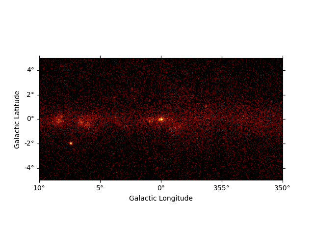
To make the structures in the image more visible we will smooth the data using a Gaussian kernel.
gc_3fhl_smoothed = gc_3fhl.smooth(kernel="gauss", width=0.2 * u.deg)
gc_3fhl_smoothed.plot(stretch="sqrt")
plt.show()
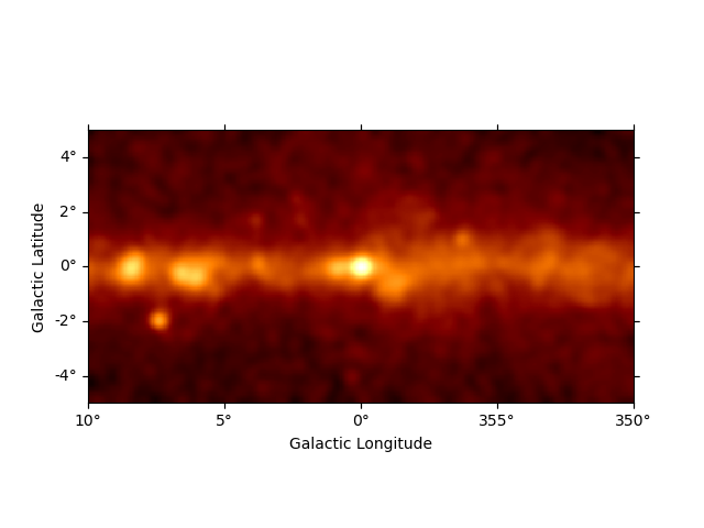
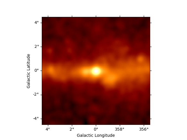
The smoothed plot already looks much nicer, but still the image is
rather large. As we are mostly interested in the inner part of the
image, we will cut out a quadratic region of the size 9 deg x 9 deg
around Vela. Therefore we use cutout to make a
cutout map:
# define center and size of the cutout region
center = SkyCoord(0, 0, unit="deg", frame="galactic")
gc_3fhl_cutout = gc_3fhl_smoothed.cutout(center, 9 * u.deg)
gc_3fhl_cutout.plot(stretch="sqrt")
plt.show()
For a more detailed introduction to maps, take a look a the
Maps notebook.
Exercises#
Add a marker and circle at the position of
Sgr A*(you can find examples in astropy.visualization.wcsaxes).
Event lists#
Almost any high level gamma-ray data analysis starts with the raw
measured counts data, which is stored in event lists. In Gammapy event
lists are represented by the EventList class.
In this section we will learn how to:
Read event lists from FITS files
Access and work with the
EventListattributes such as.tableand.energyFilter events lists using convenience methods
Let’s start with the import from the data submodule:
from gammapy.data import EventList
Very similar to the sky map class an event list can be created, by
passing a filename to the read() method:
events_3fhl = EventList.read("$GAMMAPY_DATA/fermi-3fhl-gc/fermi-3fhl-gc-events.fits.gz")
This time the actual data is stored as an
It can be accessed with `.table`` attribute:
print(events_3fhl.table)
  ENERGY      RA       DEC          L           B         THETA      PHI     ... CONVERSION_TYPE      LIVETIME      DIFRSP0 DIFRSP1 DIFRSP2 DIFRSP3 DIFRSP4
   MeV       deg       deg         deg         deg         deg       deg     ...                         s
--------- --------- ---------- ----------- ------------ --------- ---------- ... --------------- ------------------ ------- ------- ------- ------- -------
12186.642 260.45935 -33.553337   353.36273    1.7538676 71.977325  125.50694 ...               0 238.57837238907814     0.0     0.0     0.0     0.0     0.0
25496.598 261.37506 -34.395004   353.09607    0.6520652  42.49406  278.49347 ...               1 176.16850754618645     0.0     0.0     0.0     0.0     0.0
15621.498 259.56973 -33.409416   353.05673    2.4450684  64.32412  234.22194 ...               1  9.392075657844543     0.0     0.0     0.0     0.0     0.0
 12816.32 273.95883 -25.340391     6.45856   -4.0548873 43.292503  142.87392 ...               1  4.034786552190781     0.0     0.0     0.0     0.0     0.0
18988.387  260.8568 -36.355804   351.23734 -0.101912394 26.916113  290.39337 ...               0 131.60132896900177     0.0     0.0     0.0     0.0     0.0
 11610.23 266.15518 -26.224436   2.1986027    1.6034819  35.77363  274.53387 ...               1  74.98110938072205     0.0     0.0     0.0     0.0     0.0
13960.802 271.44742 -29.615316   1.6267247   -4.1431155 25.917883   238.0368 ...               1 106.37336817383766     0.0     0.0     0.0     0.0     0.0
10477.372  266.3981  -28.96814   359.97003 -0.011748177 39.091587   275.5457 ...               0 214.62817406654358     0.0     0.0     0.0     0.0     0.0
 13030.88 271.70428 -20.632627     9.59348  0.026241468 52.622505   161.3205 ...               0  94.68753063678741     0.0     0.0     0.0     0.0     0.0
11517.904 265.00894 -30.065119   358.40112   0.43904436 41.812317  276.02448 ...               0 123.15007302165031     0.0     0.0     0.0     0.0     0.0
19958.182 263.31854 -37.094856   351.71606    -2.153713 52.544586 121.415764 ...               0 17.113530546426773     0.0     0.0     0.0     0.0     0.0
 23760.14  265.4694  -31.55994   357.34256     -0.68805  52.70319  248.87813 ...               1  225.2544113099575     0.0     0.0     0.0     0.0     0.0
32168.988 266.35397 -30.096745   358.98682  -0.56723064 64.830696  212.93645 ...               1  45.64776709675789     0.0     0.0     0.0     0.0     0.0
  10165.9 266.15427 -19.829279    7.668937    4.9320326  51.85829   207.0177 ...               0 204.40402576327324     0.0     0.0     0.0     0.0     0.0
25277.545 269.68344 -24.668644   5.1628966  -0.34179303  42.77833  129.13857 ...               0  85.29761010408401     0.0     0.0     0.0     0.0     0.0
 223713.7  261.1885 -31.794796    355.1619     2.239802  25.89418   284.8728 ...               0 166.99824661016464     0.0     0.0     0.0     0.0     0.0
15236.758 264.52255 -31.730831    356.7694  -0.09604572 51.646976  141.44576 ...               0  5.334206968545914     0.0     0.0     0.0     0.0     0.0
36314.297 264.79855 -31.116806   357.41434  0.032732587 48.567314 122.824875 ...               1  34.09180650115013     0.0     0.0     0.0     0.0     0.0
 76511.96 269.20724 -26.198639   3.6230083   -0.7352153  54.72039  123.64289 ...               1  136.5931620001793     0.0     0.0     0.0     0.0     0.0
12432.439 266.09735  -32.71295   356.64053   -1.7461345 29.718775  225.30495 ...               0  57.99910423159599     0.0     0.0     0.0     0.0     0.0
14717.576 265.82196  -26.15737   2.0991938    1.8933698 50.693916  254.33784 ...               0  8.511121690273285     0.0     0.0     0.0     0.0     0.0
13233.963  269.8945 -23.260023    6.480208   0.19310227 45.217796  147.76228 ...               1 133.37614086270332     0.0     0.0     0.0     0.0     0.0
      ...       ...        ...         ...          ...       ...        ... ...             ...                ...     ...     ...     ...     ...     ...
  10941.6 265.99457 -28.765705   359.95795    0.3953491  53.88634  132.83992 ...               0 170.03486621379852     0.0     0.0     0.0     0.0     0.0
 45478.75  271.7975  -22.14616    8.313876   -0.7867925  64.49326  140.47731 ...               1 164.58107435703278     0.0     0.0     0.0     0.0     0.0
 13280.59 260.05453  -36.33665   350.88586    0.4406751  42.26522  219.64531 ...               1 22.002596974372864     0.0     0.0     0.0     0.0     0.0
74033.305 268.76508  -24.43612    4.944724    0.4974049   51.1174  225.20499 ...               0  65.83160126209259     0.0     0.0     0.0     0.0     0.0
47114.324 266.99127 -28.421051  0.70769924   -0.1726071  60.81272  212.27025 ...               1  77.02012866735458     0.0     0.0     0.0     0.0     0.0
 14473.36 259.55792 -32.497227   353.79837    2.9774146  69.47437  136.79776 ...               0 13.922565162181854     0.0     0.0     0.0     0.0     0.0
20056.527 267.50372 -21.494694    6.888726    2.9924572 46.228405  129.99919 ...               1 115.29787397384644     0.0     0.0     0.0     0.0     0.0
10021.135 266.58603 -29.006046 0.023192262  -0.17183326 58.983257  139.42741 ...               0 115.27116513252258     0.0     0.0     0.0     0.0     0.0
11217.242 260.67258 -32.080307   354.67896    2.4407566  76.96116  214.30273 ...               1  64.04110872745514     0.0     0.0     0.0     0.0     0.0
 18494.64  267.2745 -36.705185    353.7175   -4.6370916 38.942596  226.92189 ...               1 111.12007641792297     0.0     0.0     0.0     0.0     0.0
13333.997 265.57535 -31.519987   357.42413   -0.7436878  43.89681  230.49913 ...               1 23.238793969154358     0.0     0.0     0.0     0.0     0.0
13160.466 269.90778 -24.671898   5.2616706  -0.52015543   60.9269  226.45708 ...               0 1.9516496658325195     0.0     0.0     0.0     0.0     0.0
387834.72  270.3779  -21.56711    8.171749   0.64531475 56.755512  221.84715 ...               0 34.214694023132324     0.0     0.0     0.0     0.0     0.0
 20559.74  268.5538 -26.345692    3.200638  -0.30328986 49.523575  233.67285 ...               0 103.17629969120026     0.0     0.0     0.0     0.0     0.0
27209.146 266.59344  -30.52607   358.72775  -0.96718174   62.1856  140.27434 ...               0  43.22334712743759     0.0     0.0     0.0     0.0     0.0
13911.061 269.30997 -27.239439   2.7684028   -1.3365301  65.15399  224.52101 ...               0  95.46356403827667     0.0     0.0     0.0     0.0     0.0
13226.425 265.16287 -27.344238   0.7796942    1.7680178  59.38332   126.7019 ...               1  3.733097553253174     0.0     0.0     0.0     0.0     0.0
17445.463 266.63342 -28.807201  0.21464892   -0.1039705  55.48627  135.59155 ...               1  80.52235281467438     0.0     0.0     0.0     0.0     0.0
13133.864 270.42474 -22.651058    7.251185  0.071358204 48.704975  134.73102 ...               1 117.88173341751099     0.0     0.0     0.0     0.0     0.0
32095.705  266.0002  -29.77206    359.1034  -0.13615231 45.013103  236.72498 ...               0 108.92976492643356     0.0     0.0     0.0     0.0     0.0
18465.783 266.39728 -29.105953   359.85202  -0.08294058  55.97552  135.87787 ...               0  70.72638684511185     0.0     0.0     0.0     0.0     0.0
 14457.25 262.72217 -34.388405    353.7184  -0.26906812 45.683174  237.74162 ...               0  147.4274787902832     0.0     0.0     0.0     0.0     0.0
Length = 32843 rows
You can do len over event_3fhl.table to find the total number of events.
print(len(events_3fhl.table))
32843
And we can access any other attribute of the Table object as well:
print(events_3fhl.table.colnames)
['ENERGY', 'RA', 'DEC', 'L', 'B', 'THETA', 'PHI', 'ZENITH_ANGLE', 'EARTH_AZIMUTH_ANGLE', 'TIME', 'EVENT_ID', 'RUN_ID', 'RECON_VERSION', 'CALIB_VERSION', 'EVENT_CLASS', 'EVENT_TYPE', 'CONVERSION_TYPE', 'LIVETIME', 'DIFRSP0', 'DIFRSP1', 'DIFRSP2', 'DIFRSP3', 'DIFRSP4']
For convenience we can access the most important event parameters as
properties on the EventList objects. The attributes will return
corresponding Astropy objects to represent the data, such as
Quantity,
SkyCoord
or
Time
objects:
print(events_3fhl.energy.to("GeV"))
[12.186643 25.4966 15.621499 ... 32.095707 18.465784 14.457251] GeV
print(events_3fhl.galactic)
# events_3fhl.radec
<SkyCoord (Galactic): (l, b) in deg
    [(353.36228879,  1.75408483), (353.09562941,  0.6522806 ),
     (353.05628243,  2.44528685), ..., (359.10295505, -0.1359316 ),
     (359.85157506, -0.08269984), (353.71795506, -0.26883694)]>
print(events_3fhl.time)
[54682.82946153 54682.89243456 54682.89709472 ... 57236.75267735
 57233.37455141 57233.44802852]
In addition EventList provides convenience methods to filter the
event lists. One possible use case is to find the highest energy event
within a radius of 0.5 deg around the vela position:
# select all events within a radius of 0.5 deg around center
from gammapy.utils.regions import SphericalCircleSkyRegion

region = SphericalCircleSkyRegion(center, radius=0.5 * u.deg)
events_gc_3fhl = events_3fhl.select_region(region)

# sort events by energy
events_gc_3fhl.table.sort("ENERGY")

# and show highest energy photon
print("highest energy photon: ", events_gc_3fhl.energy[-1].to("GeV"))
highest energy photon: 1917.85925 GeV
Exercises#
Make a counts energy spectrum for the galactic center region, within a radius of 10 deg.
Source catalogs#
Gammapy provides a convenient interface to access and work with catalog based data.
In this section we will learn how to:
Load builtins catalogs from
catalogSort and index the underlying Astropy tables
Access data from individual sources
Let’s start with importing the 3FHL catalog object from the
catalog submodule:
from gammapy.catalog import SourceCatalog3FHL
First we initialize the Fermi-LAT 3FHL catalog and directly take a look
at the .table attribute:
fermi_3fhl = SourceCatalog3FHL()
print(fermi_3fhl.table)
   Source_Name     RAJ2000  DEJ2000    GLON     GLAT   Conf_95_SemiMajor ...           ASSOC2           ASSOC_PROB_BAY ASSOC_PROB_LR Redshift     NuPeak_obs
                     deg      deg      deg      deg           deg        ...                                                                          Hz
------------------ -------- -------- -------- -------- ----------------- ... -------------------------- -------------- ------------- -------- ------------------
3FHL J0001.2-0748    0.3107  -7.8075  89.0094 -67.3118            0.0424 ...                                    0.9974        0.9721       --  306196370000000.0
3FHL J0001.9-4155    0.4849 -41.9303 334.1216 -72.0697            0.1018 ...                                    0.9960        0.0000       -- 6309576500000000.0
3FHL J0002.1-6728    0.5283 -67.4825 310.0868 -48.9549            0.0357 ...                                    0.0000        0.9395       -- 4466832000000000.0
3FHL J0003.3-5248    0.8300 -52.8150 318.9245 -62.7936            0.0425 ...                                    0.9996        0.9716       --       7.079464e+16
3FHL J0007.0+7303    1.7647  73.0560 119.6625  10.4666            0.0101 ...                                    1.0000        0.0000       --                 --
3FHL J0007.9+4711    1.9931  47.1920 115.3093 -15.0354            0.0196 ...                                    1.0000        0.9873   0.2800 2511884200000000.0
3FHL J0008.4-2339    2.1243 -23.6514  50.2908 -79.7021            0.0366 ...                                    0.9996        0.9673   0.1470  524807800000000.0
3FHL J0009.1+0628    2.2874   6.4814 104.4637 -54.8669            0.0385 ...                                    0.9993        0.9878       --  663742400000000.0
3FHL J0009.4+5030    2.3504  50.5049 116.1257 -11.8105            0.0176 ...                                    1.0000        0.9698       -- 1412536400000000.0
3FHL J0009.7-4319    2.4450 -43.3195 327.7563 -71.7445            0.0496 ...                                    0.9985        0.9072       --                 --
3FHL J0013.0-3956    3.2523 -39.9381 332.3835 -74.9150            0.0517 ...                                    0.9998        0.9962       --    1862089000000.0
3FHL J0013.8-1855    3.4684 -18.9169  74.5314 -78.0876            0.0485 ...                                    0.9995        0.9772   0.0950       5.260181e+16
3FHL J0014.0-5024    3.5038 -50.4003 317.4913 -65.6568            0.0597 ...                                    0.9998        0.8923       --       8.413936e+16
3FHL J0014.7+5801    3.6951  58.0244 118.0788  -4.5015            0.0266 ...                                    1.0000        0.9778       --      4.3651522e+16
3FHL J0014.9+6118    3.7366  61.3025 118.5645  -1.2594            0.0339 ...                                    0.9994        0.9996       --   12971790000000.0
3FHL J0015.7+5551    3.9337  55.8649 117.9031  -6.6579            0.0335 ...                                    1.0000        0.9832       -- 6180169000000000.0
3FHL J0018.6+2946    4.6525  29.7821 114.4798 -32.5503            0.0312 ...                                    0.9985        0.9711   0.1000      5.9156075e+16
3FHL J0019.1-8151    4.7762 -81.8621 304.3273 -35.1783            0.0439 ...                                    0.9998        0.9878       -- 1393156900000000.0
3FHL J0021.4-2550    5.3693 -25.8471  42.0637 -83.1759            0.0428 ...                                    0.9996        0.9477       --  337287200000000.0
3FHL J0021.8-5140    5.4639 -51.6755 313.7480 -64.8270            0.0321 ...                                    0.9997        0.9760       -- 4786304000000000.0
3FHL J0022.0+0006    5.5032   0.1058 107.1781 -61.8626            0.0350 ...                                    0.9999        0.9408       --       1.584896e+18
3FHL J0022.1-1855    5.5260 -18.9170  82.0109 -79.3770            0.0266 ...                                    0.9987        0.8679       -- 1348963200000000.0
               ...      ...      ...      ...      ...               ... ...                        ...            ...           ...      ...                ...
3FHL J2334.8+1431  353.7183  14.5263  96.5607 -44.3897            0.0284 ...                                    0.9999        0.9674       --  113501160000000.0
3FHL J2336.3-8427  354.0982 -84.4635 305.0370 -32.3548            0.0447 ...                                    0.0000        0.9733       --                 --
3FHL J2336.5-7620  354.1298 -76.3392 308.6093 -39.9520            0.0469 ...                                    0.9991        0.9921       --                1.0
3FHL J2338.9+2123  354.7450  21.3966 101.2522 -38.4057            0.0284 ...                                    0.9998        0.9769   0.2910  524807800000000.0
3FHL J2339.2-7404  354.8159 -74.0796 309.5087 -42.1144            0.0332 ...                                    0.9999        0.9847       --        1.56675e+16
3FHL J2339.5-0533  354.8927  -5.5577  81.3085 -62.4702            0.0448 ...                                    1.0000        0.0000       --                 --
3FHL J2340.8+8015  355.2244  80.2593 119.8457  17.8129            0.0167 ...                                    1.0000        0.9970   0.2740 3427676800000000.0
3FHL J2343.6+3439  355.9012  34.6513 107.4255 -26.1696            0.0286 ...                                    0.9998        0.9819   0.3660 1029200060000000.0
3FHL J2345.1-1554  356.2999 -15.9151  65.6780 -70.9813            0.0166 ...                                    0.9999        0.9978   0.6210   20535250000000.0
3FHL J2346.6+0705  356.6726   7.0844  95.9910 -52.3676            0.0232 ...                                    0.9999        0.9971   0.1720  568853050000000.0
3FHL J2347.0+5142  356.7688  51.7008 112.8895  -9.9116            0.0129 ...                                    1.0000        0.9985   0.0440 7079464000000000.0
3FHL J2347.9+5435  356.9805  54.5974 113.7400  -7.1368            0.0276 ...                                    0.0000        0.9766       --      2.5118841e+16
3FHL J2347.9-1630  356.9978 -16.5106  65.5355 -71.8766            0.0288 ...                                    0.9994        0.9999   0.5760    9332549000000.0
3FHL J2350.5-3006  357.6354 -30.1070  16.7759 -76.3194            0.0491 ...                                    0.9998        0.9218   0.2237 3981075200000000.0
3FHL J2351.5-7559  357.8926 -75.9890 307.6546 -40.5855            0.0650 ...                                    0.0000        0.9625       --                 --
3FHL J2352.1+1753  358.0415  17.8865 103.5764 -42.7466            0.0838 ...                                    0.9926        0.0000       -- 1737799900000000.0
3FHL J2356.2+4035  359.0746  40.5985 111.7521 -21.0732            0.0298 ...                                    0.9998        0.9199   0.1310 6309576500000000.0
3FHL J2357.4-1717  359.3690 -17.2996  68.4009 -74.1285            0.0327 ...                                    0.9999        0.9631       --       8.912525e+16
3FHL J2358.4-1808  359.6205 -18.1408  66.5520 -74.8501            0.0511 ...                                    0.0000        0.0000       --                 --
3FHL J2358.5+3829  359.6266  38.4963 111.6905 -23.2173            0.0584 ...                                    0.0000        0.9254       --                 --
3FHL J2359.1-3038  359.7760 -30.6397  12.7909 -78.0268            0.0231 ...                                    0.9999        0.9975   0.1650       2.818388e+17
3FHL J2359.3-2049  359.8293 -20.8256  58.0522 -76.5411            0.0722 ...                                    0.9894        0.9906   0.0960 4073799600000000.0
Length = 1556 rows
This looks very familiar again. The data is just stored as an
Table
object. We have all the methods and attributes of the Table object
available. E.g. we can sort the underlying table by Signif_Avg to
find the top 5 most significant sources:
# sort table by significance
fermi_3fhl.table.sort("Signif_Avg")

# invert the order to find the highest values and take the top 5
top_five_TS_3fhl = fermi_3fhl.table[::-1][:5]

# print the top five significant sources with association and source class
print(top_five_TS_3fhl[["Source_Name", "ASSOC1", "ASSOC2", "CLASS", "Signif_Avg"]])
   Source_Name               ASSOC1                     ASSOC2            CLASS  Signif_Avg
------------------ -------------------------- -------------------------- ------- ----------
3FHL J0534.5+2201  Crab Nebula                                           PWN        168.641
3FHL J1104.4+3812  Mkn 421                                               BLL        144.406
3FHL J0835.3-4510  PSR J0835-4510             Vela X field               PSR        138.801
3FHL J0633.9+1746  PSR J0633+1746                                        PSR         99.734
3FHL J1555.7+1111  PG 1553+113                                           BLL         94.411
If you are interested in the data of an individual source you can access the information from catalog using the name of the source or any alias source name that is defined in the catalog:
mkn_421_3fhl = fermi_3fhl["3FHL J1104.4+3812"]

# or use any alias source name that is defined in the catalog
mkn_421_3fhl = fermi_3fhl["Mkn 421"]
print(mkn_421_3fhl.data["Signif_Avg"])
144.40611
Exercises#
Try to load the Fermi-LAT 2FHL catalog and check the total number of sources it contains.
Select all the sources from the 2FHL catalog which are contained in the Galactic Center region. The methods
contains()andpositionsmight be helpful for this. Add markers for all these sources and try to add labels with the source names.Try to find the source class of the object at position ra=68.6803, dec=9.3331
Spectral models and flux points#
In the previous section we learned how access basic data from individual sources in the catalog. Now we will go one step further and explore the full spectral information of sources. We will learn how to:
Plot spectral models
Compute integral and energy fluxes
Read and plot flux points
As a first example we will start with the Crab Nebula:
crab_3fhl = fermi_3fhl["Crab Nebula"]
crab_3fhl_spec = crab_3fhl.spectral_model()
print(crab_3fhl_spec)
PowerLawSpectralModel

type    name     value         unit        error   min max frozen link prior
---- --------- ---------- -------------- --------- --- --- ------ ---- -----
         index 2.2202e+00                2.498e-02 nan nan  False
     amplitude 1.7132e-10 cm-2 GeV-1 s-1 3.389e-12 nan nan  False
     reference 2.2726e+01            GeV 0.000e+00 nan nan   True
The crab_3fhl_spec is an instance of the
PowerLaw2SpectralModel model, with the
parameter values and errors taken from the 3FHL catalog.
Let’s plot the spectral model in the energy range between 10 GeV and 2000 GeV:
ax_crab_3fhl = crab_3fhl_spec.plot(energy_bounds=[10, 2000] * u.GeV, energy_power=0)
plt.show()
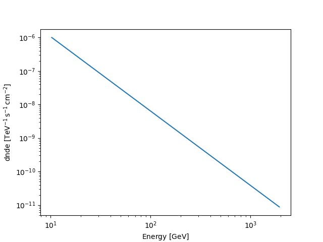
We assign the return axes object to variable called ax_crab_3fhl,
because we will re-use it later to plot the flux points on top.
To compute the differential flux at 100 GeV we can simply call the model like normal Python function and convert to the desired units:
print(crab_3fhl_spec(100 * u.GeV).to("cm-2 s-1 GeV-1"))
6.3848912826152664e-12 1 / (cm2 GeV s)
Next we can compute the integral flux of the Crab between 10 GeV and 2000 GeV:
print(
    crab_3fhl_spec.integral(energy_min=10 * u.GeV, energy_max=2000 * u.GeV).to(
        "cm-2 s-1"
    )
)
8.67457342435522e-09 1 / (cm2 s)
We can easily convince ourself, that it corresponds to the value given in the Fermi-LAT 3FHL catalog:
print(crab_3fhl.data["Flux"])
8.658909145253801e-09 1 / (cm2 s)
In addition we can compute the energy flux between 10 GeV and 2000 GeV:
print(
    crab_3fhl_spec.energy_flux(energy_min=10 * u.GeV, energy_max=2000 * u.GeV).to(
        "erg cm-2 s-1"
    )
)
5.311489174710791e-10 erg / (cm2 s)
Next we will access the flux points data of the Crab:
print(crab_3fhl.flux_points)
FluxPoints
----------

  geom                   : RegionGeom
  axes                   : ['lon', 'lat', 'energy']
  shape                  : (1, 1, 5)
  quantities             : ['norm', 'norm_errp', 'norm_errn', 'norm_ul', 'sqrt_ts', 'is_ul']
  ref. model             : pl
  n_sigma                : 1
  n_sigma_ul             : 2
  sqrt_ts_threshold_ul   : 1
  sed type init          : flux
If you want to learn more about the different flux point formats you can read the specification here.
No we can check again the underlying astropy data structure by accessing
the .table attribute:
print(crab_3fhl.flux_points.to_table(sed_type="dnde", formatted=True))
 e_ref    e_min   e_max         dnde         dnde_errp       dnde_errn        dnde_ul     sqrt_ts is_ul
  GeV      GeV     GeV    1 / (cm2 GeV s) 1 / (cm2 GeV s) 1 / (cm2 GeV s) 1 / (cm2 GeV s)
-------- ------- -------- --------------- --------------- --------------- --------------- ------- -----
  14.142  10.000   20.000       5.120e-10       1.321e-11       1.321e-11             nan 125.157 False
  31.623  20.000   50.000       7.359e-11       2.842e-12       2.842e-12             nan  88.715 False
  86.603  50.000  150.000       9.024e-12       5.367e-13       5.367e-13             nan  59.087 False
 273.861 150.000  500.000       7.660e-13       8.707e-14       8.097e-14             nan  33.076 False
1000.000 500.000 2000.000       4.291e-14       1.086e-14       9.393e-15             nan  15.573 False
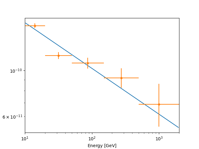
Finally let’s combine spectral model and flux points in a single plot
and scale with energy_power=2 to obtain the spectral energy
distribution:
ax = crab_3fhl_spec.plot(energy_bounds=[10, 2000] * u.GeV, sed_type="e2dnde")
crab_3fhl.flux_points.plot(ax=ax, sed_type="e2dnde")
plt.show()
Exercises#
Plot the spectral model and flux points for PKS 2155-304 for the 3FGL and 2FHL catalogs. Try to plot the error of the model (aka “Butterfly”) as well.
What next?#
This was a quick introduction to some of the high level classes in Astropy and Gammapy.
To learn more about those classes, go to the API docs (links are in the introduction at the top).
To learn more about other parts of Gammapy (e.g. Fermi-LAT and TeV data analysis), check out the other tutorial notebooks.
To see what’s available in Gammapy, browse the Gammapy docs or use the full-text search.
If you have any questions, ask on the mailing list.