Note
Go to the end to download the full example code. or to run this example in your browser via Binder
2D map fitting#
Source modelling and fitting in stacked observations using the high level interface.
Prerequisites#
To understand how a general modelling and fitting works in gammapy, please refer to the 3D detailed analysis tutorial.
Context#
We often want the determine the position and morphology of an object. To do so, we don’t necessarily have to resort to a full 3D fitting but can perform a simple image fitting, in particular, in an energy range where the PSF does not vary strongly, or if we want to explore a possible energy dependence of the morphology.
Objective#
To localize a source and/or constrain its morphology.
Proposed approach#
The first step here, as in most analysis with DL3 data, is to create
reduced datasets. For this, we will use the Analysis class to create
a single set of stacked maps with a single bin in energy (thus, an
image which behaves as a cube). This, we will then model with a
spatial model of our choice, while keeping the spectral model fixed to
an integrated power law.
# %matplotlib inline
import astropy.units as u
import matplotlib.pyplot as plt
Setup#
As usual, we’ll start with some general imports…
from IPython.display import display
from gammapy.analysis import Analysis, AnalysisConfig
Check setup#
from gammapy.utils.check import check_tutorials_setup

check_tutorials_setup()
System:

        python_executable      : /Users/mregeard/Workspace/dev/code/gammapy/gammapy/.tox/build_docs/bin/python
        python_version         : 3.11.10
        machine                : x86_64
        system                 : Darwin


Gammapy package:

        version                : 1.3.dev1205+g00f44f94ac
        path                   : /Users/mregeard/Workspace/dev/code/gammapy/gammapy/.tox/build_docs/lib/python3.11/site-packages/gammapy


Other packages:

        numpy                  : 1.26.4
        scipy                  : 1.14.1
        astropy                : 5.2.2
        regions                : 0.10
        click                  : 8.1.7
        yaml                   : 6.0.2
        IPython                : 8.28.0
        jupyterlab             : not installed
        matplotlib             : 3.9.2
        pandas                 : not installed
        healpy                 : 1.17.3
        iminuit                : 2.30.1
        sherpa                 : 4.16.1
        naima                  : 0.10.0
        emcee                  : 3.1.6
        corner                 : 2.2.2
        ray                    : 2.37.0


Gammapy environment variables:

        GAMMAPY_DATA           : /Users/mregeard/Workspace/dev/code/gammapy/gammapy-data/
Creating the config file#
Now, we create a config file for out analysis. You may load this from disc if you have a pre-defined config file.
Here, we use 3 simulated CTAO runs of the galactic center.
config = AnalysisConfig()
# Selecting the observations
config.observations.datastore = "$GAMMAPY_DATA/cta-1dc/index/gps/"
config.observations.obs_ids = [110380, 111140, 111159]
Technically, gammapy implements 2D analysis as a special case of 3D analysis (one bin in energy). So, we must specify the type of analysis as 3D, and define the geometry of the analysis.
config.datasets.type = "3d"
config.datasets.geom.wcs.skydir = {
    "lon": "0 deg",
    "lat": "0 deg",
    "frame": "galactic",
}  # The WCS geometry - centered on the galactic center
config.datasets.geom.wcs.width = {"width": "8 deg", "height": "6 deg"}
config.datasets.geom.wcs.binsize = "0.02 deg"

# The FoV radius to use for cutouts
config.datasets.geom.selection.offset_max = 2.5 * u.deg
config.datasets.safe_mask.methods = ["offset-max"]
config.datasets.safe_mask.parameters = {"offset_max": "2.5 deg"}
config.datasets.background.method = "fov_background"
config.fit.fit_range = {"min": "0.1 TeV", "max": "30.0 TeV"}

# We now fix the energy axis for the counts map - (the reconstructed energy binning)
config.datasets.geom.axes.energy.min = "0.1 TeV"
config.datasets.geom.axes.energy.max = "10 TeV"
config.datasets.geom.axes.energy.nbins = 1

config.datasets.geom.wcs.binsize_irf = "0.2 deg"

print(config)
AnalysisConfig

    general:
        log:
            level: info
            filename: null
            filemode: null
            format: null
            datefmt: null
        outdir: .
        n_jobs: 1
        datasets_file: null
        models_file: null
    observations:
        datastore: /Users/mregeard/Workspace/dev/code/gammapy/gammapy-data/cta-1dc/index/gps
        obs_ids:
        - 110380
        - 111140
        - 111159
        obs_file: null
        obs_cone:
            frame: null
            lon: null
            lat: null
            radius: null
        obs_time:
            start: null
            stop: null
        required_irf:
        - aeff
        - edisp
        - psf
        - bkg
    datasets:
        type: 3d
        stack: true
        geom:
            wcs:
                skydir:
                    frame: galactic
                    lon: 0.0 deg
                    lat: 0.0 deg
                binsize: 0.02 deg
                width:
                    width: 8.0 deg
                    height: 6.0 deg
                binsize_irf: 0.2 deg
            selection:
                offset_max: 2.5 deg
            axes:
                energy:
                    min: 0.1 TeV
                    max: 10.0 TeV
                    nbins: 1
                energy_true:
                    min: 0.5 TeV
                    max: 20.0 TeV
                    nbins: 16
        map_selection:
        - counts
        - exposure
        - background
        - psf
        - edisp
        background:
            method: fov_background
            exclusion: null
            parameters: {}
        safe_mask:
            methods:
            - offset-max
            parameters:
                offset_max: 2.5 deg
        on_region:
            frame: null
            lon: null
            lat: null
            radius: null
        containment_correction: true
    fit:
        fit_range:
            min: 0.1 TeV
            max: 30.0 TeV
    flux_points:
        energy:
            min: null
            max: null
            nbins: null
        source: source
        parameters:
            selection_optional: all
    excess_map:
        correlation_radius: 0.1 deg
        parameters: {}
        energy_edges:
            min: null
            max: null
            nbins: null
    light_curve:
        time_intervals:
            start: null
            stop: null
        energy_edges:
            min: null
            max: null
            nbins: null
        source: source
        parameters:
            selection_optional: all
    metadata:
        creator: Gammapy 1.3.dev1205+g00f44f94ac
        date: '2024-10-11T13:07:24.691100'
        origin: null
Getting the reduced dataset#
We now use the config file and create a single MapDataset containing
counts, background, exposure, psf and edisp maps.
analysis = Analysis(config)
analysis.get_observations()
analysis.get_datasets()

print(analysis.datasets["stacked"])
/Users/mregeard/Workspace/dev/code/gammapy/gammapy/.tox/build_docs/lib/python3.11/site-packages/astropy/units/core.py:2097: UnitsWarning: '1/s/MeV/sr' did not parse as fits unit: Numeric factor not supported by FITS If this is meant to be a custom unit, define it with 'u.def_unit'. To have it recognized inside a file reader or other code, enable it with 'u.add_enabled_units'. For details, see https://docs.astropy.org/en/latest/units/combining_and_defining.html
  warnings.warn(msg, UnitsWarning)
MapDataset
----------

  Name                            : stacked

  Total counts                    : 85625
  Total background counts         : 85624.99
  Total excess counts             : 0.01

  Predicted counts                : 85625.00
  Predicted background counts     : 85624.99
  Predicted excess counts         : nan

  Exposure min                    : 8.46e+08 m2 s
  Exposure max                    : 2.14e+10 m2 s

  Number of total bins            : 120000
  Number of fit bins              : 96602

  Fit statistic type              : cash
  Fit statistic value (-2 log(L)) : nan

  Number of models                : 0
  Number of parameters            : 0
  Number of free parameters       : 0
The counts and background maps have only one bin in reconstructed energy. The exposure and IRF maps are in true energy, and hence, have a different binning based upon the binning of the IRFs. We need not bother about them presently.
print(analysis.datasets["stacked"].counts)

print(analysis.datasets["stacked"].background)

print(analysis.datasets["stacked"].exposure)
WcsNDMap

        geom  : WcsGeom
        axes  : ['lon', 'lat', 'energy']
        shape : (400, 300, 1)
        ndim  : 3
        unit  :
        dtype : float32

WcsNDMap

        geom  : WcsGeom
        axes  : ['lon', 'lat', 'energy']
        shape : (400, 300, 1)
        ndim  : 3
        unit  :
        dtype : float32

WcsNDMap

        geom  : WcsGeom
        axes  : ['lon', 'lat', 'energy_true']
        shape : (400, 300, 16)
        ndim  : 3
        unit  : m2 s
        dtype : float32
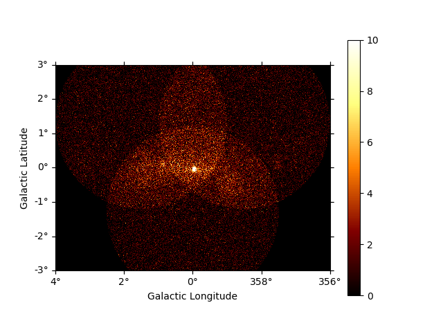
We can have a quick look of these maps in the following way:
analysis.datasets["stacked"].counts.reduce_over_axes().plot(vmax=10, add_cbar=True)
plt.show()
Modelling#
Now, we define a model to be fitted to the dataset. The important thing to note here is the dummy spectral model - an integrated powerlaw with only free normalisation. Here, we use its YAML definition to load it:
model_config = """
components:
- name: GC-1
  type: SkyModel
  spatial:
    type: PointSpatialModel
    frame: galactic
    parameters:
    - name: lon_0
      value: 0.02
      unit: deg
    - name: lat_0
      value: 0.01
      unit: deg
  spectral:
    type: PowerLaw2SpectralModel
    parameters:
    - name: amplitude
      value: 1.0e-12
      unit: cm-2 s-1
    - name: index
      value: 2.0
      unit: ''
      frozen: true
    - name: emin
      value: 0.1
      unit: TeV
      frozen: true
    - name: emax
      value: 10.0
      unit: TeV
      frozen: true
"""

analysis.set_models(model_config)
We will freeze the parameters of the background
analysis.datasets["stacked"].background_model.parameters["tilt"].frozen = True

# To run the fit
analysis.run_fit()

# To see the best fit values along with the errors
display(analysis.models.to_parameters_table())
   model    type    name      value      unit     error      min        max    frozen link prior
----------- ---- --------- ----------- -------- --------- ---------- --------- ------ ---- -----
       GC-1      amplitude  4.1624e-11 cm-2 s-1 2.220e-12        nan       nan  False
       GC-1          index  2.0000e+00          0.000e+00        nan       nan   True
       GC-1           emin  1.0000e-01      TeV 0.000e+00        nan       nan   True
       GC-1           emax  1.0000e+01      TeV 0.000e+00        nan       nan   True
       GC-1          lon_0 -5.4639e-02      deg 1.996e-03        nan       nan  False
       GC-1          lat_0 -4.6394e-02      deg 1.980e-03 -9.000e+01 9.000e+01  False
stacked-bkg           norm  9.9441e-01          3.411e-03        nan       nan  False
stacked-bkg           tilt  0.0000e+00          0.000e+00        nan       nan   True
stacked-bkg      reference  1.0000e+00      TeV 0.000e+00        nan       nan   True