Note
Go to the end to download the full example code. or to run this example in your browser via Binder
1D spectrum simulation#
Simulate a number of spectral on-off observations of a source with a power-law spectral model using the CTA 1DC response and fit them with the assumed spectral model.
Prerequisites#
Knowledge of spectral extraction and datasets used in gammapy, see for instance the spectral analysis tutorial
Context#
To simulate a specific observation, it is not always necessary to simulate the full photon list. For many uses cases, simulating directly a reduced binned dataset is enough: the IRFs reduced in the correct geometry are combined with a source model to predict an actual number of counts per bin. The latter is then used to simulate a reduced dataset using Poisson probability distribution.
This can be done to check the feasibility of a measurement, to test whether fitted parameters really provide a good fit to the data etc.
Here we will see how to perform a 1D spectral simulation of a CTAO observation, in particular, we will generate OFF observations following the template background stored in the CTAO IRFs.
Objective: simulate a number of spectral ON-OFF observations of a source with a power-law spectral model with CTAO using the CTA 1DC response, fit them with the assumed spectral model and check that the distribution of fitted parameters is consistent with the input values.
Proposed approach#
We will use the following classes and functions:
import numpy as np
import astropy.units as u
from astropy.coordinates import Angle, SkyCoord
from regions import CircleSkyRegion

# %matplotlib inline
import matplotlib.pyplot as plt
Setup#
from IPython.display import display
from gammapy.data import FixedPointingInfo, Observation, observatory_locations
from gammapy.datasets import Datasets, SpectrumDataset, SpectrumDatasetOnOff
from gammapy.irf import load_irf_dict_from_file
from gammapy.makers import SpectrumDatasetMaker
from gammapy.maps import MapAxis, RegionGeom
from gammapy.modeling import Fit
from gammapy.modeling.models import PowerLawSpectralModel, SkyModel
Check setup#
from gammapy.utils.check import check_tutorials_setup

check_tutorials_setup()
System:

        python_executable      : /Users/mregeard/Workspace/dev/code/gammapy/gammapy/.tox/build_docs/bin/python
        python_version         : 3.11.10
        machine                : x86_64
        system                 : Darwin


Gammapy package:

        version                : 1.3.dev1205+g00f44f94ac
        path                   : /Users/mregeard/Workspace/dev/code/gammapy/gammapy/.tox/build_docs/lib/python3.11/site-packages/gammapy


Other packages:

        numpy                  : 1.26.4
        scipy                  : 1.14.1
        astropy                : 5.2.2
        regions                : 0.10
        click                  : 8.1.7
        yaml                   : 6.0.2
        IPython                : 8.28.0
        jupyterlab             : not installed
        matplotlib             : 3.9.2
        pandas                 : not installed
        healpy                 : 1.17.3
        iminuit                : 2.30.1
        sherpa                 : 4.16.1
        naima                  : 0.10.0
        emcee                  : 3.1.6
        corner                 : 2.2.2
        ray                    : 2.37.0


Gammapy environment variables:

        GAMMAPY_DATA           : /Users/mregeard/Workspace/dev/code/gammapy/gammapy-data/
Simulation of a single spectrum#
To do a simulation, we need to define the observational parameters like
the livetime, the offset, the assumed integration radius, the energy
range to perform the simulation for and the choice of spectral model. We
then use an in-memory observation which is convolved with the IRFs to
get the predicted number of counts. This is Poisson fluctuated using
the fake() to get the simulated counts for each observation.
# Define simulation parameters parameters
livetime = 1 * u.h

pointing_position = SkyCoord(0, 0, unit="deg", frame="galactic")
# We want to simulate an observation pointing at a fixed position in the sky.
# For this, we use the `FixedPointingInfo` class
pointing = FixedPointingInfo(
    fixed_icrs=pointing_position.icrs,
)
offset = 0.5 * u.deg

# Reconstructed and true energy axis
energy_axis = MapAxis.from_edges(
    np.logspace(-0.5, 1.0, 10), unit="TeV", name="energy", interp="log"
)
energy_axis_true = MapAxis.from_edges(
    np.logspace(-1.2, 2.0, 31), unit="TeV", name="energy_true", interp="log"
)

on_region_radius = Angle("0.11 deg")

center = pointing_position.directional_offset_by(
    position_angle=0 * u.deg, separation=offset
)
on_region = CircleSkyRegion(center=center, radius=on_region_radius)

# Define spectral model - a simple Power Law in this case
model_simu = PowerLawSpectralModel(
    index=3.0,
    amplitude=2.5e-12 * u.Unit("cm-2 s-1 TeV-1"),
    reference=1 * u.TeV,
)
print(model_simu)
# we set the sky model used in the dataset
model = SkyModel(spectral_model=model_simu, name="source")
PowerLawSpectralModel

type    name     value         unit        error   min max frozen link prior
---- --------- ---------- -------------- --------- --- --- ------ ---- -----
         index 3.0000e+00                0.000e+00 nan nan  False
     amplitude 2.5000e-12 cm-2 s-1 TeV-1 0.000e+00 nan nan  False
     reference 1.0000e+00            TeV 0.000e+00 nan nan   True
Load the IRFs In this simulation, we use the CTA-1DC IRFs shipped with Gammapy.
irfs = load_irf_dict_from_file(
    "$GAMMAPY_DATA/cta-1dc/caldb/data/cta/1dc/bcf/South_z20_50h/irf_file.fits"
)

location = observatory_locations["cta_south"]
obs = Observation.create(
    pointing=pointing,
    livetime=livetime,
    irfs=irfs,
    location=location,
)
print(obs)
/Users/mregeard/Workspace/dev/code/gammapy/gammapy/.tox/build_docs/lib/python3.11/site-packages/astropy/units/core.py:2097: UnitsWarning: '1/s/MeV/sr' did not parse as fits unit: Numeric factor not supported by FITS If this is meant to be a custom unit, define it with 'u.def_unit'. To have it recognized inside a file reader or other code, enable it with 'u.add_enabled_units'. For details, see https://docs.astropy.org/en/latest/units/combining_and_defining.html
  warnings.warn(msg, UnitsWarning)
Observation

        obs id            : 0
        tstart            : 51544.00
        tstop             : 51544.04
        duration          : 3600.00 s
        pointing (icrs)   : 266.4 deg, -28.9 deg

        deadtime fraction : 0.0%
Simulate a spectra
# Make the SpectrumDataset
geom = RegionGeom.create(region=on_region, axes=[energy_axis])

dataset_empty = SpectrumDataset.create(
    geom=geom, energy_axis_true=energy_axis_true, name="obs-0"
)
maker = SpectrumDatasetMaker(selection=["exposure", "edisp", "background"])

dataset = maker.run(dataset_empty, obs)

# Set the model on the dataset, and fake
dataset.models = model
dataset.fake(random_state=42)
print(dataset)
SpectrumDataset
---------------

  Name                            : obs-0

  Total counts                    : 298
  Total background counts         : 22.29
  Total excess counts             : 275.71

  Predicted counts                : 303.66
  Predicted background counts     : 22.29
  Predicted excess counts         : 281.37

  Exposure min                    : 2.53e+08 m2 s
  Exposure max                    : 1.77e+10 m2 s

  Number of total bins            : 9
  Number of fit bins              : 9

  Fit statistic type              : cash
  Fit statistic value (-2 log(L)) : -1811.58

  Number of models                : 1
  Number of parameters            : 3
  Number of free parameters       : 2

  Component 0: SkyModel

    Name                      : source
    Datasets names            : None
    Spectral model type       : PowerLawSpectralModel
    Spatial  model type       :
    Temporal model type       :
    Parameters:
      index                         :      3.000   +/-    0.00
      amplitude                     :   2.50e-12   +/- 0.0e+00 1 / (cm2 s TeV)
      reference             (frozen):      1.000       TeV
You can see that background counts are now simulated
On-Off analysis#
To do an on off spectral analysis, which is the usual science case, the
standard would be to use SpectrumDatasetOnOff, which uses the
acceptance to fake off-counts. Please also refer to the Dataset simulations
section in the Spectral analysis with energy-dependent directional cuts tutorial,
dealing with simulations based on observations of real off counts.
dataset_on_off = SpectrumDatasetOnOff.from_spectrum_dataset(
    dataset=dataset, acceptance=1, acceptance_off=5
)
dataset_on_off.fake(npred_background=dataset.npred_background())
print(dataset_on_off)
SpectrumDatasetOnOff
--------------------

  Name                            : 8gaBuRdL

  Total counts                    : 286
  Total background counts         : 20.20
  Total excess counts             : 265.80

  Predicted counts                : 301.27
  Predicted background counts     : 19.90
  Predicted excess counts         : 281.37

  Exposure min                    : 2.53e+08 m2 s
  Exposure max                    : 1.77e+10 m2 s

  Number of total bins            : 9
  Number of fit bins              : 9

  Fit statistic type              : wstat
  Fit statistic value (-2 log(L)) : 7.06

  Number of models                : 1
  Number of parameters            : 3
  Number of free parameters       : 2

  Component 0: SkyModel

    Name                      : source
    Datasets names            : None
    Spectral model type       : PowerLawSpectralModel
    Spatial  model type       :
    Temporal model type       :
    Parameters:
      index                         :      3.000   +/-    0.00
      amplitude                     :   2.50e-12   +/- 0.0e+00 1 / (cm2 s TeV)
      reference             (frozen):      1.000       TeV

    Total counts_off                : 101
  Acceptance                      : 9
  Acceptance off                  : 45
You can see that off counts are now simulated as well. We now simulate several spectra using the same set of observation conditions.
n_obs = 100
datasets = Datasets()

for idx in range(n_obs):
    dataset_on_off.fake(random_state=idx, npred_background=dataset.npred_background())
    dataset_fake = dataset_on_off.copy(name=f"obs-{idx}")
    dataset_fake.meta_table["OBS_ID"] = [idx]
    datasets.append(dataset_fake)

table = datasets.info_table()
display(table)
 name  counts excess      sqrt_ts           background           npred        ...      stat_sum     counts_off acceptance   acceptance_off         alpha
                                                                              ...
------ ------ ------ ------------------ ------------------ ------------------ ... ----------------- ---------- ---------- ----------------- -------------------
 obs-0    317  298.6  27.08240194504323 18.400000000000002  68.16666666666667 ... 738.7245908429609         92        9.0              45.0                 0.2
 obs-1    275  253.0  23.76785365487285               22.0  64.16666666666669 ...  575.779512784738        110        9.0              45.0                 0.2
 obs-2    293  272.4  25.17110555404655               20.6               66.0 ... 645.4993824075303        103        9.0              45.0                 0.2
 obs-3    280  257.6 23.982951737405354               22.4  65.33333333333334 ... 585.9241546985872        112        9.0 45.00000000000001 0.19999999999999998
 obs-4    337  316.4 27.682709945184747               20.6  73.33333333333334 ...  787.314723949448        103        9.0              45.0                 0.2
 obs-5    283  258.6 23.727154782347895 24.400000000000002  67.50000000000001 ... 574.8525737727499        122        9.0              45.0                 0.2
 obs-6    330  307.6 26.889184475727866 22.400000000000006  73.66666666666667 ... 734.2414755285937        112        9.0 44.99999999999999 0.20000000000000004
 obs-7    283  257.2  23.43087974795853               25.8  68.66666666666667 ... 552.3698779448044        129        9.0              45.0                 0.2
 obs-8    308  284.6  25.42049273328331 23.400000000000002  70.83333333333334 ... 652.2621572567633        117        9.0              45.0                 0.2
 obs-9    299  278.6  25.57085071486863               20.4  66.83333333333334 ... 666.9062670260786        102        9.0 45.00000000000001 0.19999999999999998
obs-10    310  294.8 27.488972161356774               15.2  64.33333333333334 ... 768.5404492529331         76        9.0 45.00000000000001 0.19999999999999998
obs-11    285  261.0 23.933833745454685 24.000000000000004  67.50000000000001 ...  583.448753292733        120        9.0 44.99999999999999 0.20000000000000004
obs-12    299  278.0   25.4325263895117 21.000000000000004  67.33333333333336 ... 655.2768246480357        105        9.0 44.99999999999999 0.20000000000000004
obs-13    309  287.4 25.877406235012618               21.6  69.50000000000001 ...  672.355748274336        108        9.0              45.0                 0.2
obs-14    320  297.4  26.28282602819255 22.599999999999998  72.16666666666667 ... 697.5949745415169        113        9.0 45.00000000000001 0.19999999999999998
obs-15    283  261.0  24.25408979304137               22.0  65.50000000000001 ... 592.8754563739889        110        9.0              45.0                 0.2
obs-16    298  273.8 24.664218201697352 24.200000000000003  69.83333333333336 ... 619.2584188386805        121        9.0              45.0                 0.2
obs-17    301  272.8  24.01180151925227 28.200000000000003  73.66666666666667 ... 588.4976379504056        141        9.0              45.0                 0.2
obs-18    311  289.2 25.947476976949815               21.8               70.0 ... 682.6250308750984        109        9.0              45.0                 0.2
obs-19    280  257.6 23.982951737405376 22.400000000000002  65.33333333333334 ... 590.9995649814329        112        9.0              45.0                 0.2
obs-20    327  304.2  26.63324286828024 22.800000000000004  73.50000000000003 ... 720.4840155823279        114        9.0 44.99999999999999 0.20000000000000004
obs-21    286  266.8  25.08332073068164               19.2  63.66666666666668 ... 637.0646310076313         96        9.0 45.00000000000001 0.19999999999999998
   ...    ...    ...                ...                ...                ... ...               ...        ...        ...               ...                 ...
obs-78    337  314.4  27.23331180179332               22.6  75.00000000000001 ... 750.4026293749382        113        9.0              45.0                 0.2
obs-79    315  294.6   26.4957236283439               20.4               69.5 ... 711.0546046139739        102        9.0 45.00000000000001 0.19999999999999998
obs-80    304  282.8  25.67868740385823 21.200000000000003  68.33333333333336 ... 669.9654389755506        106        9.0 44.99999999999999 0.20000000000000004
obs-81    301  281.6 25.922347414834622 19.400000000000002  66.33333333333334 ... 678.9813616402096         97        9.0              45.0                 0.2
obs-82    280  258.0 24.072587044084237 22.000000000000004               65.0 ... 581.8610083160877        110        9.0 44.99999999999999 0.20000000000000004
obs-83    303  280.8 25.394928282299105 22.200000000000003  69.00000000000001 ... 654.4650896470343        111        9.0 44.99999999999999 0.20000000000000004
obs-84    269  247.8 23.580247140026987 21.200000000000003 62.500000000000014 ... 577.2362891766269        106        9.0 44.99999999999999 0.20000000000000004
obs-85    297  274.6 24.998935845735573               22.4  68.16666666666667 ... 631.6298361198053        112        9.0 45.00000000000001 0.19999999999999998
obs-86    286  268.2  25.42340896951546 17.800000000000004  62.50000000000001 ... 655.2082535886425         89        9.0 44.99999999999999 0.20000000000000004
obs-87    333  313.2 27.646851451147217               19.8  72.00000000000001 ... 770.1313412321031         99        9.0              45.0                 0.2
obs-88    315  296.8   27.0172059251097 18.200000000000003  67.66666666666669 ... 734.6476098262428         91        9.0 44.99999999999999 0.20000000000000004
obs-89    287  265.0  24.49456558680515 22.000000000000004  66.16666666666667 ... 611.2334063685089        110        9.0 44.99999999999999 0.20000000000000004
obs-90    286  267.0 25.131221887043438 19.000000000000004  63.50000000000001 ... 635.8304116110406         95        9.0 44.99999999999999 0.20000000000000004
obs-91    285  259.8  23.67754591931069 25.200000000000003  68.50000000000001 ... 573.3564742963381        126        9.0              45.0                 0.2
obs-92    313  289.4 25.664935420194176               23.6  71.83333333333336 ... 669.4496142825196        118        9.0              45.0                 0.2
obs-93    302  283.2 26.123867522605497               18.8  66.00000000000001 ... 700.5066738339824         94        9.0              45.0                 0.2
obs-94    322  300.2 26.574029757473202               21.8  71.83333333333334 ... 715.2570498037147        109        9.0              45.0                 0.2
obs-95    305  280.6 25.030731260493152 24.400000000000006  71.16666666666667 ... 643.2846879404793        122        9.0 44.99999999999999 0.20000000000000004
obs-96    301  277.4 24.969845969421428               23.6  69.83333333333334 ... 626.7396842428624        118        9.0              45.0                 0.2
obs-97    290  271.2 25.417982194454826               18.8  64.00000000000001 ... 650.9762484493856         94        9.0              45.0                 0.2
obs-98    301  280.6 25.687832964675007 20.400000000000002  67.16666666666667 ... 664.5620099404952        102        9.0              45.0                 0.2
obs-99    323  302.2  26.85707842376871               20.8  71.16666666666669 ... 733.1576598768017        104        9.0              45.0                 0.2
Length = 100 rows
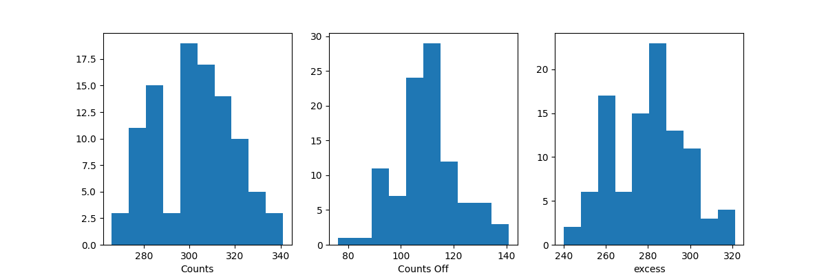
Before moving on to the fit let’s have a look at the simulated observations.
Now, we fit each simulated spectrum individually
results = []

fit = Fit()

for dataset in datasets:
    dataset.models = model.copy()
    result = fit.optimize(dataset)
    results.append(
        {
            "index": result.parameters["index"].value,
            "amplitude": result.parameters["amplitude"].value,
        }
    )
We take a look at the distribution of the fitted indices. This matches very well with the spectrum that we initially injected.
fig, ax = plt.subplots()
index = np.array([_["index"] for _ in results])
ax.hist(index, bins=10, alpha=0.5)
ax.axvline(x=model_simu.parameters["index"].value, color="red")
ax.set_xlabel("Reconstructed spectral index")
print(f"index: {index.mean()} += {index.std()}")
plt.show()
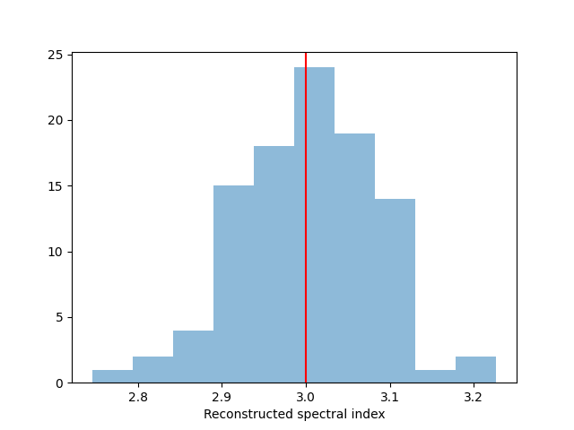
index: 3.0036925550377753 += 0.08081469527631224
Exercises#
Change the observation time to something longer or shorter. Does the observation and spectrum results change as you expected?
Change the spectral model, e.g. add a cutoff at 5 TeV, or put a steep-spectrum source with spectral index of 4.0
Simulate spectra with the spectral model we just defined. How much observation duration do you need to get back the injected parameters?