Note
Go to the end to download the full example code. or to run this example in your browser via Binder
Source detection and significance maps#
Build a list of significant excesses in a Fermi-LAT map.
Context#
The first task in a source catalog production is to identify significant excesses in the data that can be associated to unknown sources and provide a preliminary parametrization in terms of position, extent, and flux. In this notebook we will use Fermi-LAT data to illustrate how to detect candidate sources in counts images with known background.
Objective: build a list of significant excesses in a Fermi-LAT map
Proposed approach#
This notebook show how to do source detection with Gammapy using the
methods available in estimators. We will use images from a
Fermi-LAT 3FHL high-energy Galactic center dataset to do this:
perform adaptive smoothing on counts image
produce 2-dimensional test-statistics (TS)
run a peak finder to detect point-source candidates
compute Li & Ma significance images
estimate source candidates radius and excess counts
Note that what we do here is a quick-look analysis, the production of real source catalogs use more elaborate procedures.
We will work with the following functions and classes:
Setup#
As always, let’s get started with some setup …
import numpy as np
import astropy.units as u

# %matplotlib inline
import matplotlib.pyplot as plt
from IPython.display import display
from gammapy.datasets import MapDataset
from gammapy.estimators import ASmoothMapEstimator, TSMapEstimator
from gammapy.estimators.utils import find_peaks, find_peaks_in_flux_map
from gammapy.irf import EDispKernelMap, PSFMap
from gammapy.maps import Map
from gammapy.modeling.models import PointSpatialModel, PowerLawSpectralModel, SkyModel
Check setup#
from gammapy.utils.check import check_tutorials_setup

check_tutorials_setup()
System:

        python_executable      : /Users/mregeard/Workspace/dev/code/gammapy/gammapy/.tox/build_docs/bin/python
        python_version         : 3.11.10
        machine                : x86_64
        system                 : Darwin


Gammapy package:

        version                : 1.3.dev1205+g00f44f94ac
        path                   : /Users/mregeard/Workspace/dev/code/gammapy/gammapy/.tox/build_docs/lib/python3.11/site-packages/gammapy


Other packages:

        numpy                  : 1.26.4
        scipy                  : 1.14.1
        astropy                : 5.2.2
        regions                : 0.10
        click                  : 8.1.7
        yaml                   : 6.0.2
        IPython                : 8.28.0
        jupyterlab             : not installed
        matplotlib             : 3.9.2
        pandas                 : not installed
        healpy                 : 1.17.3
        iminuit                : 2.30.1
        sherpa                 : 4.16.1
        naima                  : 0.10.0
        emcee                  : 3.1.6
        corner                 : 2.2.2
        ray                    : 2.37.0


Gammapy environment variables:

        GAMMAPY_DATA           : /Users/mregeard/Workspace/dev/code/gammapy/gammapy-data/
Read in input images#
We first read the relevant maps:
counts = Map.read("$GAMMAPY_DATA/fermi-3fhl-gc/fermi-3fhl-gc-counts-cube.fits.gz")
background = Map.read(
    "$GAMMAPY_DATA/fermi-3fhl-gc/fermi-3fhl-gc-background-cube.fits.gz"
)

exposure = Map.read("$GAMMAPY_DATA/fermi-3fhl-gc/fermi-3fhl-gc-exposure-cube.fits.gz")

psfmap = PSFMap.read(
    "$GAMMAPY_DATA/fermi-3fhl-gc/fermi-3fhl-gc-psf-cube.fits.gz",
    format="gtpsf",
)

edisp = EDispKernelMap.from_diagonal_response(
    energy_axis=counts.geom.axes["energy"],
    energy_axis_true=exposure.geom.axes["energy_true"],
)

dataset = MapDataset(
    counts=counts,
    background=background,
    exposure=exposure,
    psf=psfmap,
    name="fermi-3fhl-gc",
    edisp=edisp,
)
/Users/mregeard/Workspace/dev/code/gammapy/gammapy/.tox/build_docs/lib/python3.11/site-packages/astropy/wcs/wcs.py:803: FITSFixedWarning: 'datfix' made the change 'Set DATEREF to '2001-01-01T00:01:04.184' from MJDREF.
Set MJD-OBS to 54682.655283 from DATE-OBS.
Set MJD-END to 57236.967546 from DATE-END'.
  warnings.warn(
Adaptive smoothing#
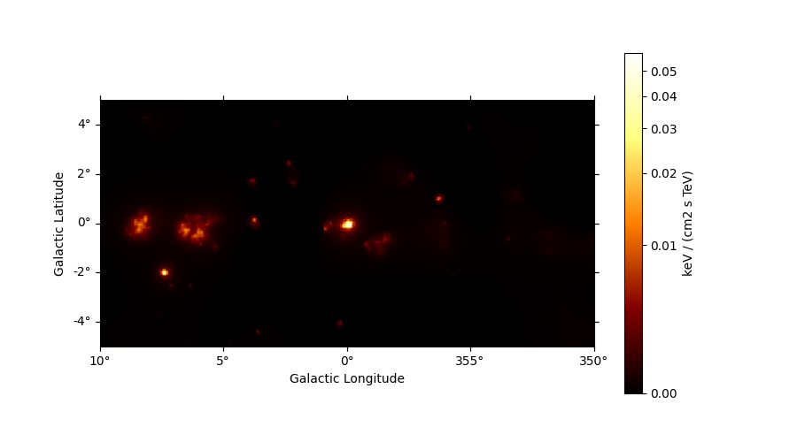
For visualisation purpose it can be nice to look at a smoothed counts image. This can be performed using the adaptive smoothing algorithm from Ebeling et al. (2006).
In the following example the ASmoothMapEstimator.threshold argument gives the minimum
significance expected, values below are clipped.
scales = u.Quantity(np.arange(0.05, 1, 0.05), unit="deg")
smooth = ASmoothMapEstimator(threshold=3, scales=scales, energy_edges=[10, 500] * u.GeV)
images = smooth.run(dataset)

plt.figure(figsize=(9, 5))
images["flux"].plot(add_cbar=True, stretch="asinh")
plt.show()
TS map estimation#
The Test Statistic, \(TS = 2 \Delta log L\) (Mattox et al. 1996), compares the likelihood function L optimized with and without a given source. The TS map is computed by fitting by a single amplitude parameter on each pixel as described in Appendix A of Stewart (2009). The fit is simplified by finding roots of the derivative of the fit statistics (default settings use Brent’s method).
We first need to define the model that will be used to test for the existence of a source. Here, we use a point source.
spatial_model = PointSpatialModel()

# We choose units consistent with the map units here...
spectral_model = PowerLawSpectralModel(amplitude="1e-22 cm-2 s-1 keV-1", index=2)
model = SkyModel(spatial_model=spatial_model, spectral_model=spectral_model)
Here we show a full configuration of the estimator. We remind the user of the meaning of the various quantities:
model: aSkyModelwhich is converted to a source model kernelkernel_width: the width for the above kerneln_sigma: number of sigma for the flux errorn_sigma_ul: the number of sigma for the flux upper limitsselection_optional: what optional maps to computen_jobs: for running in parallel, the number of processes used for the computationsum_over_energy_groups: to sum over the energy groups or fit thenormon the full energy cube
estimator = TSMapEstimator(
    model=model,
    kernel_width="1 deg",
    energy_edges=[10, 500] * u.GeV,
    n_sigma=1,
    n_sigma_ul=2,
    selection_optional=None,
    n_jobs=1,
    sum_over_energy_groups=True,
)


maps = estimator.run(dataset)
Accessing and visualising results#
Below we print the result of the TSMapEstimator. We have access to a number of
different quantities, as shown below. We can also access the quantities names
through map_result.available_quantities.
print(maps)
FluxMaps
--------

  geom                   : WcsGeom
  axes                   : ['lon', 'lat', 'energy']
  shape                  : (400, 200, 1)
  quantities             : ['ts', 'norm', 'niter', 'norm_err', 'npred', 'npred_excess', 'stat', 'stat_null', 'success']
  ref. model             : pl
  n_sigma                : 1
  n_sigma_ul             : 2
  sqrt_ts_threshold_ul   : 2
  sed type init          : likelihood
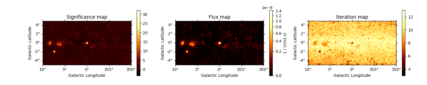
fig, (ax1, ax2, ax3) = plt.subplots(
    ncols=3,
    figsize=(20, 3),
    subplot_kw={"projection": counts.geom.wcs},
    gridspec_kw={"left": 0.1, "right": 0.98},
)

maps["sqrt_ts"].plot(ax=ax1, add_cbar=True)
ax1.set_title("Significance map")
maps["flux"].plot(ax=ax2, add_cbar=True, stretch="sqrt", vmin=0)
ax2.set_title("Flux map")
maps["niter"].plot(ax=ax3, add_cbar=True)
ax3.set_title("Iteration map")
plt.show()
The flux in each pixel is obtained by multiplying a reference model with a normalisation factor:
print(maps.reference_model)
SkyModel

  Name                      : 0aBSteC3
  Datasets names            : None
  Spectral model type       : PowerLawSpectralModel
  Spatial  model type       : PointSpatialModel
  Temporal model type       :
  Parameters:
    index                         :      2.000   +/-    0.00
    amplitude                     :   1.00e-22   +/- 0.0e+00 1 / (cm2 keV s)
    reference             (frozen):      1.000       TeV
    lon_0                         :      0.000   +/-    0.00 deg
    lat_0                         :      0.000   +/-    0.00 deg
maps.norm.plot(add_cbar=True, stretch="sqrt")
plt.show()
Source candidates#
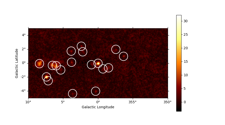
Let’s run a peak finder on the sqrt_ts image to get a list of
point-sources candidates (positions and peak sqrt_ts values). The
find_peaks function performs a local maximum search in a sliding
window, the argument min_distance is the minimum pixel distance
between peaks (smallest possible value and default is 1 pixel).
sources = find_peaks(maps["sqrt_ts"], threshold=5, min_distance="0.25 deg")
nsou = len(sources)
display(sources)

# Plot sources on top of significance sky image
plt.figure(figsize=(9, 5))
ax = maps["sqrt_ts"].plot(add_cbar=True)

ax.scatter(
    sources["ra"],
    sources["dec"],
    transform=ax.get_transform("icrs"),
    color="none",
    edgecolor="w",
    marker="o",
    s=600,
    lw=1.5,
)
plt.show()

# sphinx_gallery_thumbnail_number = 3
value   x   y      ra       dec
                  deg       deg
------ --- --- --------- ---------
32.194 200  99 266.41449 -28.97054
27.833  52  60 272.43197 -23.54282
 15.16  32  98 271.16056 -21.74479
14.134  69  93 270.40919 -23.47797
13.872  80  92 270.15899 -23.98049
9.7638 273 119 263.18257 -31.52587
 8.793 124 102 268.46711 -25.63326
7.3491 123 134 266.97596 -24.77174
6.8071 193  19 270.59696 -30.69138
6.2432 152 148 265.48068 -25.64323
5.8704 230  86 266.15140 -30.58926
5.6678 127  12 272.77351 -27.97934
5.6557 251 139 262.90685 -30.05853
5.4712 181  95 267.17020 -28.26173
5.4209 214  83 266.78188 -29.98429
5.1736  57  49 272.82739 -24.02653
 5.067 156 132 266.12148 -26.23306
5.0414  93  80 270.37773 -24.84233
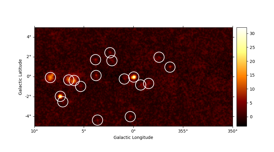
We can also utilise find_peaks_in_flux_map
to display various parameters from the FluxMaps
sources_flux_map = find_peaks_in_flux_map(maps, threshold=5, min_distance="0.25 deg")
display(sources_flux_map)
 x   y      ra       dec        ts        norm   niter norm_err   npred    npred_excess    stat    stat_null  success     flux      flux_err
           deg       deg                                                                                              1 / (cm2 s) 1 / (cm2 s)
--- --- --------- --------- ---------- --------- ----- -------- ---------- ------------ ---------- ---------- ------- ----------- -----------
 93  80 270.37773 -24.84233   25.41555   8.27043   8.0  2.37914  290.78937     27.07074  815.20556  840.62111    True   8.105e-11   2.332e-11
156 132 266.12148 -26.23306   25.67442   6.00005   8.0  1.89724  155.88363     19.73494  666.92009  692.59451    True   5.880e-11   1.859e-11
 57  49 272.82739 -24.02653   26.76643   5.68610   7.0  1.76385  106.04843     18.55966  696.93904  723.70546    True   5.572e-11   1.729e-11
214  83 266.78188 -29.98429   29.38654   9.89249   9.0  2.63543  450.31686     32.72392  809.50127  838.88781    True   9.695e-11   2.583e-11
181  95 267.17020 -28.26173   29.93437  13.12076   9.0  3.22925  697.64626     43.25799  629.45787  659.39224    True   1.286e-10   3.165e-11
251 139 262.90685 -30.05853   31.98741   6.79990   8.0  1.95252  174.09938     22.54051  734.23408  766.22149    True   6.664e-11   1.913e-11
127  12 272.77351 -27.97934   32.12432   4.19126   8.0  1.37638   62.78010     13.76505  401.25085  433.37517    True   4.107e-11   1.349e-11
230  86 266.15140 -30.58926   34.46172  13.03987   9.0  3.10155  500.87813     43.20346  831.08719  865.54892    True   1.278e-10   3.040e-11
152 148 265.48068 -25.64323   38.97700   7.22434   8.0  1.91470  140.64858     23.74536  572.78773  611.76473    True   7.080e-11   1.876e-11
193  19 270.59696 -30.69138   46.33614   6.74666   8.0  1.74591   90.43161     22.28446  398.95343  445.28958    True   6.612e-11   1.711e-11
123 134 266.97596 -24.77174   54.00972   9.39519   7.0  2.16644  159.65186     30.82310  601.76247  655.77218    True   9.207e-11   2.123e-11
124 102 268.46711 -25.63326   77.31675  17.36545   9.0  3.11225  434.86369     56.97380  804.66583  881.98258    True   1.702e-10   3.050e-11
273 119 263.18257 -31.52587   95.33086  17.99310   8.0  3.00754  396.20281     59.75164  751.59404  846.92490    True   1.763e-10   2.947e-11
 80  92 270.15899 -23.98049  192.41910  46.69483   8.0  5.38562  494.88697    152.68893  901.04315 1093.46225    True   4.576e-10   5.278e-11
 69  93 270.40919 -23.47797  199.75682  46.45624   8.0  5.36583  507.14543    151.74287  844.50081 1044.25763    True   4.553e-10   5.259e-11
 32  98 271.16056 -21.74479  229.82409  55.11421   7.0  5.91212  539.20902    179.26857  806.59952 1036.42361    True   5.401e-10   5.794e-11
 52  60 272.43197 -23.54282  774.66618  61.05926   7.0  4.76383  318.62545    199.21166  317.75376 1092.41995    True   5.984e-10   4.669e-11
200  99 266.41449 -28.97054 1036.45364 144.33603   7.0  8.05908 1096.56231    476.57624 -899.15077  137.30287    True   1.414e-09   7.898e-11
Note that we used the instrument point-spread-function (PSF) as kernel, so the hypothesis we test is the presence of a point source. In order to test for extended sources we would have to use as kernel an extended template convolved by the PSF. Alternatively, we can compute the significance of an extended excess using the Li & Ma formalism, which is faster as no fitting is involve.
What next?#
In this notebook, we have seen how to work with images and compute TS and significance images from counts data, if a background estimate is already available.
Here’s some suggestions what to do next:
Look how background estimation is performed for IACTs with and without the high level interface in High level interface and Low level API notebooks, respectively
Learn about 2D model fitting in the 2D map fitting notebook
Find more about Fermi-LAT data analysis in the Fermi-LAT with Gammapy notebook
Use source candidates to build a model and perform a 3D fitting (see 3D detailed analysis, Multi instrument joint 3D and 1D analysis notebooks for some hints)
Total running time of the script: (0 minutes 12.589 seconds)